Lab 05: Schlieren Imaging & Supersonic Wind Tunnels

Experiment Overview

Shock waves are one of the most dramatic phenomena in compressible flow — a razor-thin region where pressure, temperature, and density jump discontinuously. They appear inside nozzles, around supersonic bodies, and at control surface impingement points. Schlieren imaging makes them visible without touching the flow, an elegant optical technique used in supersonic aircraft testing, ballistic research, and scramjet development. This lab introduced blowdown supersonic wind tunnel operation and applied Schlieren photography to characterize a normal shock inside the nozzle.

• Understand the operating cycle and components of a blowdown supersonic wind tunnel
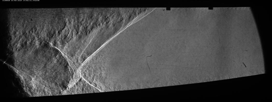
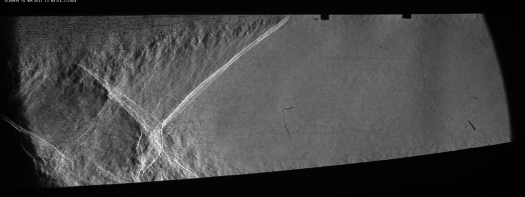
• Use Schlieren optics to visually locate and characterize a normal shock in the diverging nozzle section
• Compute the nozzle pressure ratio (NPR) and shock strength from 13 static pressure taps
• Determine the choked-flow mass flow rate through the nozzle throat

Equipment & Tools

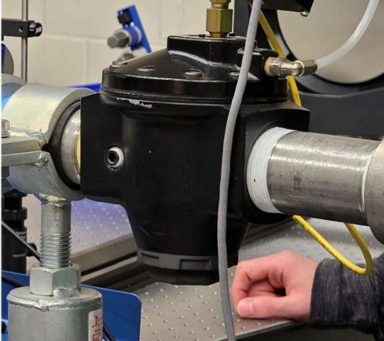
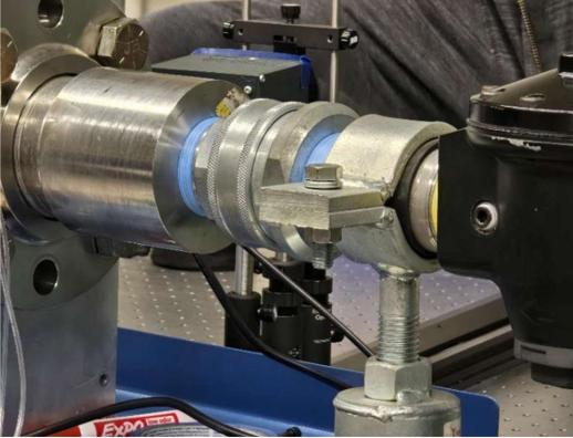
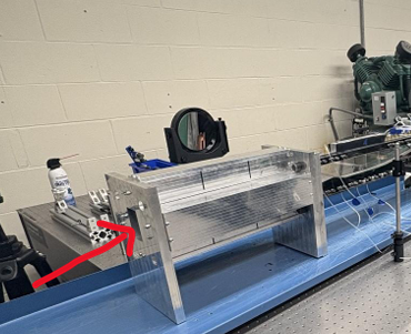
• ERAU blowdown supersonic wind tunnel with convergent-divergent nozzle (A_throat = 0.765 in², half-angle ≈4.8°)
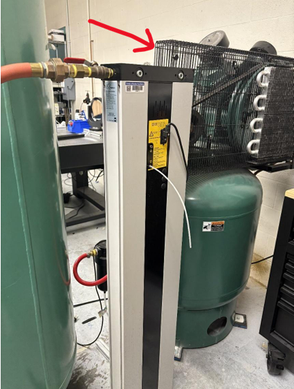
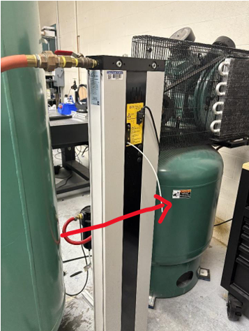
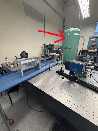
• Air compressor, high-pressure storage tank, main valve, and pressure regulator
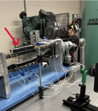
• 13 static pressure taps along the nozzle floor (positions 1.5–19.5 inches)
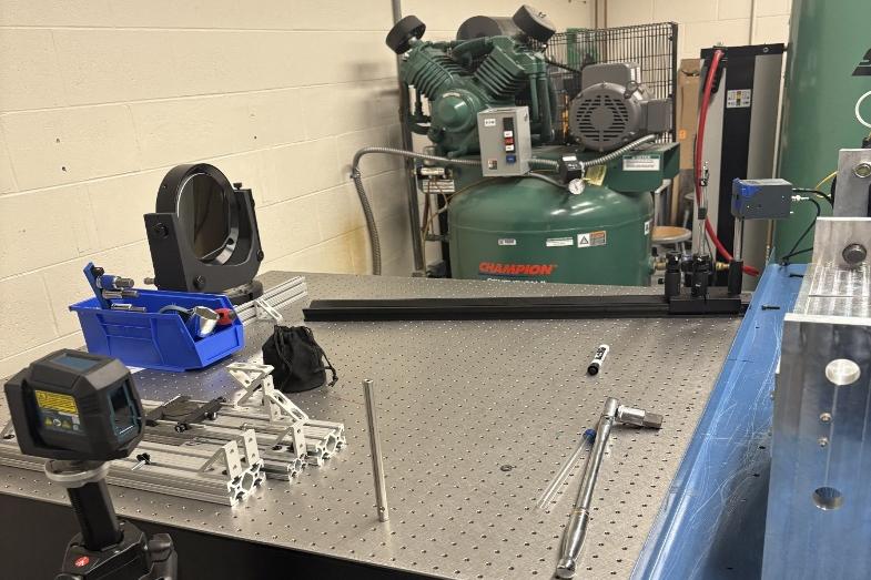
• Schlieren optical imaging system (mirrors, point light source, razor blade cutoff, digital camera)
• Wind tunnel silencer and quick-disconnect nozzle
• TracerDAQ data acquisition software; MATLAB for pressure analysis

Approach & Key Equations

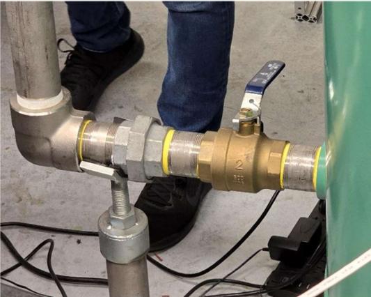
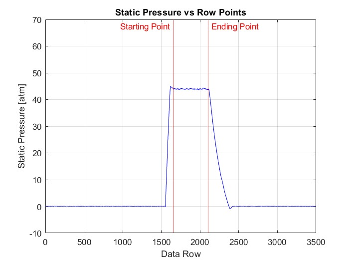
The ERAU blowdown tunnel stores compressed air, releases it through a pressure regulator into a convergent-divergent nozzle, and exhausts through a silencer. Thirteen static taps sampled the floor pressure distribution during steady-state operation (identified from the time history as rows 1,653–2,103). Total pressure was back-calculated at the throat assuming Mach 1 flow, and the nozzle pressure ratio was compared against the critical value to confirm shock presence:

NPR = P₀ / P_exit     Shock strength S = P_after / P_before

Mass flow rate was computed from isentropic choked-flow theory. Schlieren images were captured simultaneously to visually confirm shock position and morphology.

Key Results

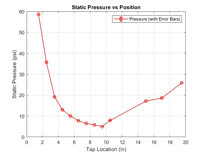
• Schlieren images confirmed a clear normal shock between tap positions 9.5 and 10.5 inches in the diverging section — exactly where static pressure data showed an abrupt pressure rise.
• NPR = 3.932 — exceeding the critical NPR, confirming the flow was choked at the throat and a shock existed inside the nozzle.
• Shock strength S = 1.614 — a 61.4% pressure jump across the shock, classifying it as a moderately strong normal shock.
• Mass flow rate = 6.10 lbm/s through the 0.765 in² throat, consistent with the measured stagnation conditions from choked-flow theory.
• The pressure trace showed the textbook normal shock signature: a smooth decrease through the diverging section, a sharp spike at the shock, and recovery to near back pressure downstream.

MATLAB Code

Raw pressure data was time-averaged over the steady-state window, augmented with atmospheric pressure, and used to back-calculate total pressure and compute NPR, shock strength, and mass flow rate.

% Steady-state average + atmospheric correction
range_ss  = tempData(1653:2103, :);
dataframe = mean(range_ss) + Patm;       % 13 taps (psi)

% Back-calculate total pressure from throat (M = 1)
P0    = dataframe(2) / (1 + (y-1)/2)^(-y/(y-1));

% NPR and shock strength
NPR   = P0 / mean(dataframe(11));        % = 3.932
shock = dataframe(10) / dataframe(9);    % = 1.614  (S = P_after/P_before)

% Choked-flow mass rate (lbm/s)
a    = sqrt(y * R * T);
mdot = Ath * (P0/a) * sqrt(y) * ((2/(y+1))^((y+1)/(2*(y-1)))) * 32.174;

Valuable Takeaways

• Schlieren imaging turns invisible physics into a photograph. Seeing a shock wave in an actual image — not just a textbook diagram — makes the density gradient concept tangible. The technique is widely used in supersonic testing, hypersonic wind tunnels, and shock-tube experiments.
• NPR is the single diagnostic quantity for nozzle flow regime. Knowing whether NPR exceeds the critical value tells an engineer immediately whether the throat is choked and a shock is present — essential knowledge for nozzle design in rocket engines and high-speed inlets.
• Normal shocks are lossy — they create entropy. The shock strength of 1.614 represents an irreversible pressure rise that drives designers toward oblique shocks and shock-management systems in real supersonic inlets.
• Gained hands-on experience with a blowdown supersonic facility, interpreted Schlieren photography, and applied compressible flow relations to extract propulsion-relevant parameters from instrumentation data.